Conditional Formatting (5)
Lists and ranges (5)
Macros (VBA procedures) (63)
Miscellaneous (39)
Excel bugs and glitches (4)

How to find a value in another table or VLOOKUP strength

In fact, in this article I want to talk about the possibilities not only VLOOKUP functions, but I also want to touch on SEARCH, as a function very related to VPR. Each of these functions has both its pros and cons. In a nutshell, VLOOKUP searches for a certain value we specify among the many values located in one column. Perhaps most often the need for VLOOKUP arises when you need to compare data, find data in another table, add data from one table to another, based on some criterion, etc.
To understand the principle of VLOOKUP a little better, it’s better to start with some practical example. There is a table like this:
Fig.1

and from the first table must be substituted into the second date for each surname. For three records this is not a problem and doing it manually is all obvious. But in real life, these are tables with thousands of records, and searching with data substitution manually can take more than one hour. Plus a couple more fly in the ointment: not only are the names located in completely different orders in both tables and the number of records in the tables is different, but the tables are also located on different sheets/books. I believe I have convinced you that manual substitution is not an option at all. But VLOOKUP will be indispensable here. In this case, practically nothing will need to be done - just write in the first cell of column C of the second table (where you need to substitute the dates from the first table) this formula:
=VLOOKUP($A2 ;Sheet1!$A$2:$C$4 ;3,0)
You can write a formula either directly into a cell, or using the function manager, selecting in the category Links and Arrays VPR and separately indicating the necessary criteria. Now we copy( Ctrl+C) cell with the formula, select all the cells in column C to the end of the data and insert ( Ctrl+V).

First, the basic principle of operation: VLOOKUP looks in the first column of the Table argument for the value specified by the argument Search_value . When the desired value is found, the function returns the value opposite the found value, but from the column specified by the argument Column_number . We'll deal with time-lapse viewing a little later. A VLOOKUP can only return one value - the first one that matches the criterion. If the value you are looking for is not found (not in the table), then the result of the function will be #N/A . There is no need to be afraid of this - it is even useful. You will know exactly which records are missing and thus can compare two tables with each other. Sometimes it turns out that you see: there is data in both tables, but the VLOOKUP produces #N/A. This means that the data in your tables is not identical. Some of them have extra inconspicuous spaces (usually before or after the value), or Cyrillic characters are mixed with Latin characters. Also #N/A will be if the criteria are numbers and in the desired table they are written as text (usually a green triangle appears in the upper left corner of such a cell), and in the final one - as numbers. Or vice versa.

Description of VLOOKUP arguments
$A2 - argument Search_value(let's call it Criterion to be short). This is what we are looking for. Those. for the first record of the second table it will be Petrov S.A. Here you can specify either the text of the criterion directly (in this case it should be in quotes - =VLOOKUP("Petrov S.A" ;Sheet1!$A$2:$C$4;3;0) or a link to a cell with this text (as in the function example). There is a small nuance: you can also use wildcard characters: "*" and "?". This is very convenient if you need to find values only for part of a string. For example, you may not enter “Petrov S.A” in full, but enter only the last name and the asterisk - “Petrov*”. Then any entry that begins with “Petrov” will be displayed. If you need to find a record in which the surname “Petrov” appears anywhere on the line, then you can specify it like this: “*Petrov*”. If you want to find the surname Petrov and it doesn’t matter what initials the first name and patronymic will have (if the full name is written as Ivanov I.I.), then this look is just right: “Ivanov?.?.” . Often it is necessary to indicate its value for each line (in column A Surnames and you need to find them all). In this case, references to the cells of column A are always indicated. For example, in cell A1 it is written: Ivanov. It is also known that Ivanov is in another table, but after the last name both the first and middle names (or something else) can be written down. But we only need to find the string that starts with the last name. Then you need to write it as follows: A1 &"*" . This entry will be equivalent to "Ivanov*". A1 is written Ivanov, the ampersand(&) is used to combine two text values into one string. An asterisk is in quotation marks (as text inside a formula should be). Thus we get:
A1&"*" =>
"Ivanov"&"*" =>
"Ivanov*"
Very convenient if there are a lot of values to search for.
If you need to determine whether there is a word somewhere in a line, then put asterisks on both sides: "*"& A1 &"*"

Sheet1!$A$2:$C$4 - argument Table. Specifies the range of cells. Only the range must contain data from the first data cell to the very last. This does not have to be the range shown in the example. If there are 100 rows, then Sheet1!$A$2:$C$100. It is important to remember three things: first, this Table must always start with the column in which we are looking Criterion . And nothing else. Otherwise, nothing will be found or the result will not be what you expect. Second: argument Table must be "fixed" . What does it mean. Do you see the dollar signs? This is consolidation (more precisely, this is called an absolute range reference). How it's done. Highlight link text (only one range - one criterion) and press F4 until you see that dollars appear before both the column name and the row number. If this is not done, then when copying the formula, the Table argument will “move out” and the result will again be incorrect. And lastly, the table must contain columns from the first (in which we are searching) to the last (from which we need to return values). In the example Sheet1!$A$2:$C$4- this means it will not be possible to return the value from column D(4), because the table has only three columns.

3 - Column_number. Here we simply indicate the column number in the argument Table, the values from which we need to substitute as the result. In the example, this is the Acceptance Date - i.e. column number 3. If we needed a department, then we would indicate 2, and if we just needed to compare whether there are names from one table in another, then we could specify 1. Important: argument Column_number must not exceed the number of columns in the argument Table . Otherwise the formula will result in an error #LINK!. For example, if the range $B$2:$C$4 is specified and you need to return data from column C, then it is correct to specify 2. Because argument Table($B$2:$C$4) contains only two columns - B and C. If you try to specify the number of column 3 (as it appears on the sheet), you will get an error #LINK!, because there is simply no third column in the specified range.

Practical advice: if the Table argument has too many columns and you need to return the result from the last column, then it is not at all necessary to calculate their number. You can specify it like this: =VLOOKUP($A2 ;Sheet1! $A$2:$C$4 ;COLUMN NUM(Sheet1! $A$2:$C$4);0) . By the way, in this case Sheet1! can also be removed as unnecessary: =VLOOKUP($A2 ;Sheet1! $A$2:$C$4 ;COLUMN NUM($A$2:$C$4);0) .

0 - Time-lapse_view- a very interesting argument. Can be either TRUE or FALSE. The question immediately arises: why is there 0 in my formula? It's very simple - Excel in formulas can treat 0 as FALSE and 1 as TRUE. If you specify this parameter in VLOOKUP equal to 0 or FALSE, then an exact match to the specified Criterion will be searched. This has nothing to do with wildcards ("*" and "?"). If you use 1 or TRUE (or do not specify the last argument at all, since by default it is TRUE), then... It’s a very long story. In short - VLOOKUP will look for the most similar value that matches Criterion . Sometimes very useful. However, if you use this parameter, then it is necessary that the list in the Table argument be sorted in ascending order. Please note that sorting is only necessary if the Interval_lookup argument is TRUE or 1. If it is 0 or FALSE, sorting is not needed.

Many people probably noticed that in the picture I have the departments for full names mixed up. This is not a recording error. The example attached to the article shows how you can substitute both them and dates with one formula, without manually changing the argument Column_number. It seemed to me that such an example could be quite useful.

How to avoid the #N/A (#N/A) error in VLOOKUP?
Another common problem is that many people do not want to see #N/A as a result if a match is not found. This is easy to get around:
=IF(END(VLOOKUP($A2,Sheet1! $A$2:$C$4,3,0));"";VLOOKUP($A2,Sheet1! $A$2:$C$4,3,0)))
Now if VLOOKUP does not find a match, the cell will be empty.
And users of Excel 2007 and higher versions can use IFERROR:
=IFERROR(VLOOKUP($A2,Sheet1! $A$2:$C$4,3,0);"")

The Promised MATCH

This function looks for the value specified by the parameter Search_value in argument View_array. And the result of the function is the position number of the found value in View_array. It is the position number, not the value itself. In principle, I will not describe it in the same detail, because the main points are exactly the same. If we wanted to apply it to the table above, it would be like this:
=MATCH($A2,Sheet1! $A$2:$A$4,0)
$A2 - Search_value. Here everything is exactly the same as with VLOOKUP. Wildcard characters are also allowed and in exactly the same design.

Sheet1! $A$2:$A$4 - The array to be viewed. The main difference from VLOOKUP is that you can specify an array with only one column. This should be the column we are going to search in Search_value . If you try to specify more than one column, the function will return an error.

match_type(0) - the same as in VPR Time-lapse_view . With the same features. It differs only in the ability to search for the smallest from the desired or the largest. But I will not dwell on this in this article.

We've sorted out the basics. But we need to return not the position number, but the value itself. This means that SEARCH in its pure form is not suitable for us. At least one, by itself. But if it is used together with the INDEX function, then this is what we need and even more.
=INDEX(Sheet1! $A$2:$C$4 ;MATCH($A2 ;Sheet1! $A$2:$A$4 ;0);2)
This formula will return the same result as VLOOKUP.

INDEX Function Arguments
Sheet1! $A$2:$C$4 - Array. As this argument we specify the range from which we want to get the values. There can be one column or several. If there is only one column, then the last function argument does not need to be specified. By the way, this argument may not coincide at all with the one we specify in the Lookup_array argument of the MATCH function.

Next come Row_Number and Column_Number. It is as Row_Number that we substitute MATCH, which returns us the position number in the array. This is what everything is built on. INDEX returns the value from the Array that is in the specified row(RowNumber) of the Array and the specified column(ColumnNumber) if there is more than one column. It is important to know that in this combination, the number of rows in the Array argument of the INDEX function and the number of rows in the Lookup_array argument of the MATCH function must match. And start from the same line. This is in ordinary cases, unless you are pursuing other goals.
As with VLOOKUP, INDEX returns #N/A if the desired value is not found. And you can get around such errors in the same way:
For all versions of Excel (including 2003 and earlier):
=IF(END(MATCH($A2,Sheet1! $A$2:$A$4,0));"";INDEX(Sheet1! $A$2:$C$4;MATCH($A2,Sheet1! $A$2: $A$4 ;0);2))
For versions 2007 and higher:
=IFERROR(INDEX(Sheet1! $A$2:$C$4,MATCH($A2,Sheet1!$A$2:$A$4,0),2);"")

Working with criteria longer than 255 characters
INDEX-SEARCH also has one more advantage over VLOOKUP. The point is that VLOOKUP cannot look up values the line length of which contains more than 255 characters. This happens rarely, but it does happen. You can, of course, cheat the VLOOKUP and cut down the criterion:
=VLOOKUP(PSTR($A2,1,255),PSTR(Sheet1!$A$2:$C$4,1,255),3,0)
but this is an array formula. And besides, such a formula will not always return the desired result. If the first 255 characters are identical to the first 255 characters in the table, and then the characters are different, the formula will no longer see this. And the formula returns exclusively text values, which is not very convenient in cases where numbers should be returned.

Therefore, it is better to use this tricky formula:
=INDEX(Sheet1!$A$2:$C$4,SUMPRODUCT(MATCH(TRUE,Sheet1!$A$2:$A$4 =$A2,0));2)
Here I used the same ranges in the formulas for readability, but in the example for downloading they differ from those indicated here.
The formula itself is built on the ability of the SUMPRODUCT function to transform into massive calculations of some functions within it. In this case, MATCH looks for the row position where the criterion is equal to the value in the row. Wildcard characters can no longer be used here.

In the example attached to the article you will find examples of the use of all the described cases and an example of why INDEX and MATCH are sometimes preferable to VLOOKUP.

Download example

(26.0 KiB, 14,615 downloads)

Did the article help? Share the link with your friends! Video lessons

("Bottom bar":("textstyle":"static","textpositionstatic":"bottom","textautohide":true,"textpositionmarginstatic":0,"textpositiondynamic":"bottomleft","textpositionmarginleft":24," textpositionmarginright":24,"textpositionmargintop":24,"textpositionmarginbottom":24,"texteffect":"slide","texteffecteasing":"easeOutCubic","texteffectduration":600,"texteffectslidedirection":"left","texteffectslidedistance" :30,"texteffectdelay":500,"texteffectseparate":false,"texteffect1":"slide","texteffectslidedirection1":"right","texteffectslidedistance1":120,"texteffecteasing1":"easeOutCubic","texteffectduration1":600 ,"texteffectdelay1":1000,"texteffect2":"slide","texteffectslidedirection2":"right","texteffectslidedistance2":120,"texteffecteasing2":"easeOutCubic","texteffectduration2":600,"texteffectdelay2":1500," textcss":"display:block; padding:12px; text-align:left;","textbgcss":"display:block; position:absolute; top:0px; left:0px; width:100%; height:100% ; background-color:#333333; opacity:0.6; filter:alpha(opacity=60);","titlecss":"display:block; position:relative; font:bold 14px \"Lucida Sans Unicode\",\"Lucida Grande\",sans-serif,Arial; color:#fff;","descriptioncss":"display:block; position:relative; font:12px \"Lucida Sans Unicode\",\"Lucida Grande\",sans-serif,Arial; color:#fff; margin-top:8px;","buttoncss":"display:block; position:relative; margin-top:8px;","texteffectresponsive":true,"texteffectresponsivesize":640,"titlecssresponsive":"font-size:12px;","descriptioncssresponsive":"display:none !important;","buttoncssresponsive": "","addgooglefonts":false,"googlefonts":"","textleftrightpercentforstatic":40))

Microsoft Excel often works with large amounts of information. It creates huge tables with thousands of rows, columns and positions. It can be difficult to find any specific data in such an array. And sometimes it’s completely impossible. This task can be simplified. Find out how to find the right word in Excel. This will make it easier for you to navigate the document. And you can quickly jump to the information you are looking for.

To display the addresses of all cells that contain what you are looking for, do the following:

If you have Office 2010, go to Menu - Edit - Find.
A window with an input field will open. Write a search phrase in it.
In Excel 2007, this button is on the Home menu in the Editing panel. It's on the right.
A similar result in all versions can be achieved by pressing Ctrl+F.
In the field, type the word, phrase or numbers you want to find.
Click Find All to search the entire document. If you click “Next”, the program will select the cells one by one that are located below the Excel cell cursor.
Wait for the process to finish. The larger the document, the longer the system will search.
A list will appear with the results: the names and addresses of the cells in which there are matches with the given phrase, and the text that is written in them.
When you click on each line, the corresponding cell will be highlighted.
For convenience, you can “stretch” the window. This way more lines will be visible.
To sort the data, click on the column names above the search results. If you click on “Sheet”, the lines will be arranged alphabetically depending on the name of the sheet; if you select “Values”, they will be arranged by value.
These columns also "stretch".

You can set your own conditions. For example, run a search using several characters. Here's how to find a word in Excel that you don't remember entirely:

Enter only part of the caption. You can write at least one letter - all places where it exists will be highlighted.
Use the symbols * (asterisk) and ? (question mark). They replace missing characters.
The question indicates one missing item. If you write, for example, “P???,” cells will appear that contain a four-character word that starts with “P”: “Plow,” “Field,” “Couple,” and so on.
A star (*) can replace any number of characters. To find all values that contain the root “rast”, start searching using the key “*rast*”.

You can also go to settings:

In the Find window, click Options.
In the “Browse” and “Search Area” sections, specify where and by what criteria to look for matches. You can select formulas, notes, or values.
To allow the system to distinguish between lowercase and uppercase letters, check the “Match case” checkbox.
If you check the “Entire cell” checkbox, the results will show cells that contain only the specified search phrase and nothing else.

Cell Format Options

To find values with a specific fill or style, use the settings. Here's how to find a word in Excel if it looks different from the rest of the text:

In the search window, click “Options” and click on the “Format” button. A menu with several tabs will open.
You can specify a specific font, frame type, background color, data format. The system will view places that match the specified criteria.
To take information from the current cell (currently highlighted), click "Use this cell's format." Then the program will find all values that have the same size and type of symbols, the same color, the same borders, and the like.

Search multiple words

In Excel, you can find cells by entire phrases. But if you entered the “Blue Ball” key, the system will work exactly on this request. Values with "Blue Crystal Ball" or "Blue Glitter Ball" will not appear in the results.

To find not just one word in Excel, but several at once, do the following:

Write them in the search bar.
Place stars between them. The result will be “*Text* *Text2* *Text3*”. This will find all values containing the specified inscriptions. Regardless of whether there are any characters between them or not.
This way you can specify a key even with individual letters.

Filter

Here's how to search in Excel using a filter:

Select any filled cell.
Click Home - Sort - Filter.
Arrows will appear next to the cells in the top line. This is a drop down menu. Open it.
Enter your request in the text field and click OK.
The column will only display cells that contain the search phrase.
To reset the results, select “Select all” in the drop-down list.
To disable a filter, click on it again in the sorting.

This method will not work if you do not know in which row the value you need is in.

To find a phrase or number in Excel, use the built-in interface capabilities. You can select additional search options and turn on a filter.

Batyanov Denis As a guest author, he talks in this post about how to find data in one Excel table and extract it into another, and also reveals all the secrets of the vertical view function.

Using the COLUMN function to specify the extraction column

If the table you are retrieving data into using VLOOKUP has the same structure as the lookup table, but simply contains fewer rows, then VLOOKUP can use the COLUMN() function to automatically calculate the column numbers to retrieve. In this case, all VLOOKUP formulas will be the same (adjusted for the first parameter, which changes automatically)! Please note that the first parameter has an absolute column coordinate.

Creating a composite key using &»|»&

If there is a need to search in several columns at the same time, then it is necessary to create a composite key for the search. If the returned value were not text (as is the case with the “Code” field), but numeric, then the more convenient SUMIFS formula would be suitable for this and the composite column key would not be required at all.

This is my first article for Lifehacker. If you liked it, then I invite you to visit my website, and I will also be happy to read in the comments about your secrets of using the VLOOKUP function and the like. Thank you. :)

The main purpose of the Excel office program is to perform calculations. This program's document (Book) can contain many sheets with long tables filled with numbers, text or formulas. Automated quick search allows you to find the necessary cells in them.

Simple search

To search for a value in an Excel table, you need to open the drop-down list of the Find and Replace tool on the “Home” tab and click “Find.” The same effect can be achieved using the keyboard shortcut Ctrl + F.

In the simplest case, in the “Find and Replace” window that appears, you need to enter the desired value and click “Find All”.

As you can see, search results have appeared at the bottom of the dialog box. The found values are underlined in red in the table. If instead of “Find all” you click “Find next”, then the first cell with this value will be searched first, and when you click again, the second one will be searched.

Text search is performed in the same way. In this case, the searched text is typed in the search bar.

If data or text is not searched in the entire Excel table, then the search area must first be selected.

Advanced Search

Suppose you want to find all values in the range from 3000 to 3999. In this case, you would type 3??? in the search bar. Wildcard "?" replaces any other.

Analyzing the results of the search, it can be noted that, along with the correct 9 results, the program also produced unexpected ones, highlighted in red. They are associated with the presence of the number 3 in a cell or formula.

You can be satisfied with most of the results obtained, ignoring the incorrect ones. But the search function in Excel 2010 can work much more accurately. The Options tool in the dialog box is for this purpose.

By clicking "Options", the user has the ability to perform advanced searches. First of all, let’s pay attention to the “Search Area” item, which by default is set to “Formulas”.

This means that the search was carried out, including in those cells where there is not a value, but a formula. The presence of the number 3 in them gave three incorrect results. If you select "Values" as the search scope, you will only search for data and the incorrect results associated with formula cells will disappear.

In order to get rid of the only remaining incorrect result on the first line, in the advanced search window you need to select the “Entire cell” item. After this, the search result becomes 100% accurate.

This result could be achieved by immediately selecting the “Entire Cell” item (even leaving the “Formula” value in the “Search Area”).

Now let's turn to the “Search” item.

If instead of the default “On Sheet” you select “In Workbook”, then there is no need to be on the sheet of cells you are looking for. The screenshot shows that the user initiated the search while on empty sheet 2.

The next item in the advanced search window is “View”, which has two meanings. The default is “by rows”, which means that the cells are scanned row by row. Selecting a different value – “by columns” – will only change the search direction and the sequence of results.

When searching in Microsoft Excel documents, you can use another wildcard character – “*”. If the considered "?" meant any character, then “*” replaces not one, but any number of characters. Below is a screenshot of a search for Louisiana.

Sometimes it is necessary to take into account the case of characters when searching. If the word louisiana is capitalized, the search results will not change. But if you select “Match case” in the advanced search window, the search will be unsuccessful. The program will consider the words Louisiana and louisiana different, and, naturally, will not find the first of them.

Types of search

Search for matches

Sometimes it is necessary to detect duplicate values in a table. To search for matches, you first need to select a search range. Then, on the same “Home” tab, in the “Styles” group, open the “Conditional Formatting” tool. Next, sequentially select the items “Rules for highlighting cells” and “Repeating values”.

The result is shown in the screenshot below.

If necessary, the user can change the color of the visual display of matched cells.

Filtration

Another type of search is filtering. Let's assume that the user wants to find numeric values in the range from 3000 to 4000 in column B.

As you can see, only rows that satisfy the entered condition are displayed. All the rest were temporarily hidden. To return to the initial state, repeat step 2.

Various search options were discussed using Excel 2010 as an example. How to search in Excel of other versions? There is a difference in the transition to filtering in version 2003. In the “Data” menu, you should sequentially select the commands “Filter”, “Auto Filter”, “Condition” and “Custom Auto Filter”.

Video: Search in an Excel table

Among thousands of rows and dozens of columns of data, it is almost impossible to manually find something in an Excel table. The only option is to use some kind of search function, and next we will look at how to search in an Excel table.

To search for data in an Excel table, you must use the menu item "Find and Select" on the tab "Home", in which you need to select an option "Find" or use the key combination to call "Ctrl + F".

For example, let's try to find the required number among the data in our table, since it is when searching for numbers that we need to take into account some subtleties of the search. Let's look for a number in the Excel table "10".

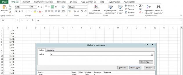
After selecting the required menu item, enter the desired value in the search box that appears. We have two options for searching values in an Excel table, this is to find all matches at once by clicking the button "Find All" or immediately view each found cell by pressing the button each time "Find Next". When using the button "Find Next" you should also take into account the current location of the active cell, since the search will begin from this position.

Let's try to find all the values at once, and everything found will be listed in the window under the search settings. If we leave all the default settings, the search result will not be exactly what we expected.

To correctly search for data in an Excel table, click the button "Options" and configure the search area. Now the desired value is searched even in the formulas used in the cells for calculations. We need to specify the search only in values and, if desired, we can also specify the format of the searched data.

When searching for words in an Excel table, you should also take into account all these subtleties and, for example, you can even take into account the case of letters.

And finally, let’s look at how to search for data in Excel only in the required area of the sheet. As can be seen from our example, the desired value "10" occurs in all data columns at once. If you need to find this value, say, only in the first column, you need to select this column or any area of values in which you need to search, and then begin the search.